Optimisation

# Copyright (C) 2020. Huawei Technologies Co., Ltd. All rights reserved.

# This program is free software; you can redistribute it and/or modify it under
# the terms of the MIT license.

# This program is distributed in the hope that it will be useful, but WITHOUT ANY
# WARRANTY; without even the implied warranty of MERCHANTABILITY or FITNESS FOR A
# PARTICULAR PURPOSE. See the MIT License for more details.

import sys
sys.path.append('../')
import pandas as pd
import matplotlib.pyplot as plt
import numpy as np
import torch
from pymoo.factory import get_problem,get_visualization


from hebo.optimizers.hebo import HEBO
from hebo.optimizers.bo import BO

import warnings
warnings.filterwarnings("ignore")

Demo problem definition

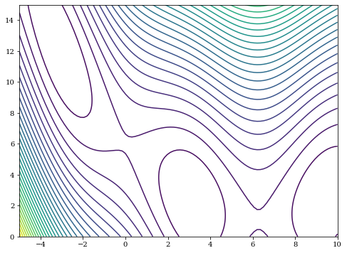
We will introduce the optimizer API using branin function defined in pymoo library

This is what branin function looks like, it has three local minima

problem = get_problem('go-branin01')

get_visualization("fitness-landscape", problem, angle=(45, 45), _type="contour").show()

<pymoo.visualization.fitness_landscape.FitnessLandscape at 0x26304e0ea88>

Objective function wrapper

The branin function is wrapped using obj(x : pd.DataFrame) -> pd.DataFrame

def obj(x : pd.DataFrame) -> np.ndarray:
    x     = x[['x0','x1']].values
    num_x = x.shape[0]
    ret   = np.zeros((num_x,1))
    for i in range(num_x):
        out = {}
        try:
            problem._evaluate(x[i], out)
        except:
            problem._evaluate(x[i].reshape(1,-1),out)
        ret[i,0] = out['F'][0]
    return ret

Design space definition

from hebo.design_space.design_space import DesignSpace
space = DesignSpace().parse([
    {'name' : 'x0', 'type' : 'num', 'lb' : -5, 'ub' : 10},
    {'name' : 'x1', 'type' : 'num', 'lb' : 0,  'ub' : 15}
])

BO loop

We compare three BO algorithms: - The basic BO with LCB acquisition - HEBO where three acquisition functions are ensembled, with input warping and power transformation - HEBO with parallel recommendation

We’ll run BO with LCB firstly, we can see the interface is very simple

bo   = BO(space)
for i in range(64):
    rec_x = bo.suggest()
    bo.observe(rec_x, obj(rec_x))
    if i % 4 == 0:
        print('Iter %d, best_y = %.2f' % (i, bo.y.min()))

Iter 0, best_y = 152.87
Iter 4, best_y = 40.28
Iter 8, best_y = 1.95
Iter 12, best_y = 0.78
Iter 16, best_y = 0.47
Iter 20, best_y = 0.42
Iter 24, best_y = 0.40
Iter 28, best_y = 0.40
Iter 32, best_y = 0.40
Iter 36, best_y = 0.40
Iter 40, best_y = 0.40
Iter 44, best_y = 0.40
Iter 48, best_y = 0.40
Iter 52, best_y = 0.40
Iter 56, best_y = 0.40
Iter 60, best_y = 0.40

We then run the sequential HEBO

hebo_seq   = HEBO(space, model_name = 'gpy', rand_sample = 4)
for i in range(64):
    rec_x = hebo_seq.suggest(n_suggestions=1)
    hebo_seq.observe(rec_x, obj(rec_x))
    if i % 4 == 0:
        print('Iter %d, best_y = %.2f' % (i, hebo_seq.y.min()))

Iter 0, best_y = 24.13
Iter 4, best_y = 18.11
Iter 8, best_y = 13.77
Iter 12, best_y = 1.16
Iter 16, best_y = 1.16
Iter 20, best_y = 0.46
Iter 24, best_y = 0.41
Iter 28, best_y = 0.41
Iter 32, best_y = 0.41
Iter 36, best_y = 0.40
Iter 40, best_y = 0.40
Iter 44, best_y = 0.40
Iter 48, best_y = 0.40
Iter 52, best_y = 0.40
Iter 56, best_y = 0.40
Iter 60, best_y = 0.40

Finally, we run the parallel HEBO, as it would do parallel recommendation, we only run it for 16 iterations

hebo_batch = HEBO(space, model_name = 'gpy', rand_sample = 4)
for i in range(16):
    rec_x = hebo_batch.suggest(n_suggestions=8)
    hebo_batch.observe(rec_x, obj(rec_x))
    print('Iter %d, best_y = %.2f' % (i, hebo_batch.y.min()))

Iter 0, best_y = 6.95
Iter 1, best_y = 0.96
Iter 2, best_y = 0.88
Iter 3, best_y = 0.43
Iter 4, best_y = 0.40
Iter 5, best_y = 0.40
Iter 6, best_y = 0.40
Iter 7, best_y = 0.40
Iter 8, best_y = 0.40
Iter 9, best_y = 0.40
Iter 10, best_y = 0.40
Iter 11, best_y = 0.40
Iter 12, best_y = 0.40
Iter 13, best_y = 0.40
Iter 14, best_y = 0.40
Iter 15, best_y = 0.40

conv_hebo_batch = np.minimum.accumulate(hebo_batch.y)
conv_hebo_seq   = np.minimum.accumulate(hebo_seq.y)
conv_bo_seq     = np.minimum.accumulate(bo.y)

We plot the converge below, we can see it seems that the LCB converges slightly faster than HEBO, while batched HEBO used most function evaluations

plt.figure(figsize = (8,6))
plt.semilogy(conv_hebo_batch - problem.ideal_point(), 'x-',label = 'HEBO, Parallel,Batch = 8')
plt.semilogy(conv_hebo_seq   - problem.ideal_point(), 'x-',label = 'HEBO, Sequential')
plt.semilogy(conv_bo_seq     - problem.ideal_point(), 'x-',label = 'BO, LCB')

plt.xlabel('Evaluation')
plt.ylabel('Regret')
plt.legend()

<matplotlib.legend.Legend at 0x274a6946908>

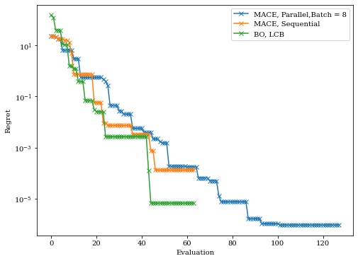
Batched HEBO used most function evaluations because it recommend eight points per iterations, we can also plot the converge against iterations instead of evaluations

plt.figure(figsize = (8,6))
plt.semilogy(conv_hebo_batch[::8] - problem.ideal_point(), 'x-',label = 'HEBO, Parallel,Batch = 8')
plt.semilogy(conv_hebo_seq   - problem.ideal_point(), 'x-',label = 'HEBO, Sequential')
plt.semilogy(conv_bo_seq     - problem.ideal_point(), 'x-',label = 'BO, LCB')

plt.xlabel('Iterations')
plt.ylabel('Regret')
plt.legend()

<matplotlib.legend.Legend at 0x274a694f508>

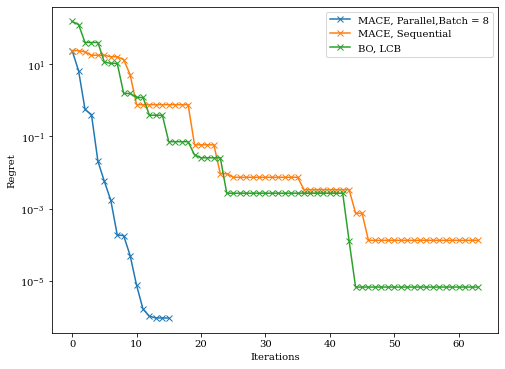
We can see that parallel HEBO converges much faster