Advanced optimisation
In this section, we show how HEBO can be used for constrained and multi-objective optimisation
Objective function
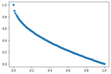
We use benchmark functions from pymoo
[1]:
import numpy as np
import torch
import pandas as pd
import matplotlib.pyplot as plt
from pymoo.factory import get_problem
from pymoo.util.plotting import plot
from pymoo.util.dominator import Dominator


problem = get_problem("zdt1", n_var = 5)
plot(problem.pareto_front())

dim = problem.n_var
num_obj = problem.n_obj
num_constr = problem.n_constr
We define a wrapper for our BO algorithm, the wrapper function takes in a pd.DataFrame and output an np.ndarray where left columns are objectives and constraint values are in right columns.
[2]:
def obj(param : pd.DataFrame) -> np.ndarray:
    names = ['x' + str(i) for i in range(problem.n_var)]
    x   = param[names].values
    out = {}
    problem._evaluate(x,out)
    o = out['F'].reshape(x.shape[0], num_obj)
    if num_constr > 0:
        c = out['G'].reshape(x.shape[0], num_constr)
    else:
        c = np.zeros((x.shape[0],0))
    return np.hstack([o,c])

def extract_pf(points : np.ndarray) -> np.ndarray:
    dom_matrix = Dominator().calc_domination_matrix(points,None)
    is_optimal = (dom_matrix >= 0).all(axis = 1)
    return points[is_optimal]
Design space
[3]:
from hebo.design_space.design_space import DesignSpace

lb,ub  = problem.bounds()
params = [{'name' : 'x' + str(i), 'type' : 'num', 'lb' : lb[i], 'ub' : ub[i]} for i in range(dim)]
space  = DesignSpace().parse(params)
space.sample(5)
[3]:
| x0 | x1 | x2 | x3 | x4 | |
|---|---|---|---|---|---|
| 0 | 0.248171 | 0.632608 | 0.240098 | 0.490050 | 0.732430 |
| 1 | 0.931607 | 0.034736 | 0.701038 | 0.516294 | 0.121251 |
| 2 | 0.645922 | 0.065483 | 0.469201 | 0.127420 | 0.123271 |
| 3 | 0.160319 | 0.797957 | 0.901810 | 0.912018 | 0.235120 |
| 4 | 0.188969 | 0.337747 | 0.181045 | 0.068357 | 0.539323 |
Bayesian optimisation
The GeneralBO class can be used to perform multi-objective bayesian optimisation
[9]:
from hebo.optimizers.general import GeneralBO
conf = {}
conf['num_hiddens'] = 64
conf['num_layers'] = 2
conf['output_noise'] = False
conf['rand_prior'] = True
conf['verbose'] = False
conf['l1'] = 3e-3
conf['lr'] = 3e-2
conf['num_epochs'] = 100
opt = GeneralBO(space, num_obj, num_constr, model_conf = conf)
for i in range(50):
    rec = opt.suggest(n_suggestions=4)
    opt.observe(rec, obj(rec))
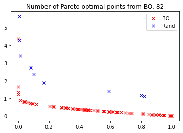
We’ll plot the Pareto front given by BO algorithm, and compare it with random search, we can see that BO gives much better PF than random search
[10]:
feasible_y = extract_pf(opt.y)
rand_y     = extract_pf(obj(space.sample(opt.y.shape[0])))
plt.plot(feasible_y[:,0], feasible_y[:,1], 'x', color = 'r', label = 'BO')
plt.plot(rand_y[:,0], rand_y[:,1], 'x', color = 'b', label = 'Rand')
plt.title('Number of Pareto optimal points from BO: %d' % feasible_y.shape[0])
plt.legend()
[10]:
<matplotlib.legend.Legend at 0x29010f9d308>
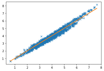
Model accuracy checking
[7]:
params = space.sample(1000)
values = obj(params)
with torch.no_grad():
    py,ps2 = opt.model.predict(*space.transform(params))
plt.plot(values[:,1], py[:,1], 'x')
plt.plot(values[:,1], values[:,1])
[7]:
[<matplotlib.lines.Line2D at 0x29010eeb488>]
Copyright statment
Copyright (C) 2020. Huawei Technologies Co., Ltd. All rights reserved.
This program is free software; you can redistribute it and/or modify it under the terms of the MIT license.
This program is distributed in the hope that it will be useful, but WITHOUT ANY WARRANTY; without even the implied warranty of MERCHANTABILITY or FITNESS FOR A PARTICULAR PURPOSE. See the MIT License for more details.